
How We Find Records When We Don’t Know Where To Look
Devising an efficient person-based flow for medical record retrieval

“How do I get my medical records?”
This is one of the most common requests in healthcare. With Datavant’s Switchboard, we are reducing the time and number of steps involved for patients to get their medical records. But patients are not the only requesters of medical records – a significant number of requests for medical records come, for example, from insurance companies making Medicare risk adjustments. In order to demonstrate that an insured population meets certain risk criteria, insurance companies must pull medical records for these patients in large numbers. Datavant only routes requests that have proper authorization and are allowable under HIPAA guidelines, a quantity which currently amounts to around 50 million record requests per year from a variety of requesters.
How are large-volume record requests fulfilled and how can we make the process faster and more reliable?
Two routes to the record: providers and patients
We need a minimum amount of information to locate a patient’s medical record. Historically, our Chart Requester product used a provider-based flow to route searches for medical records, which requires the following information to locate a medical record:
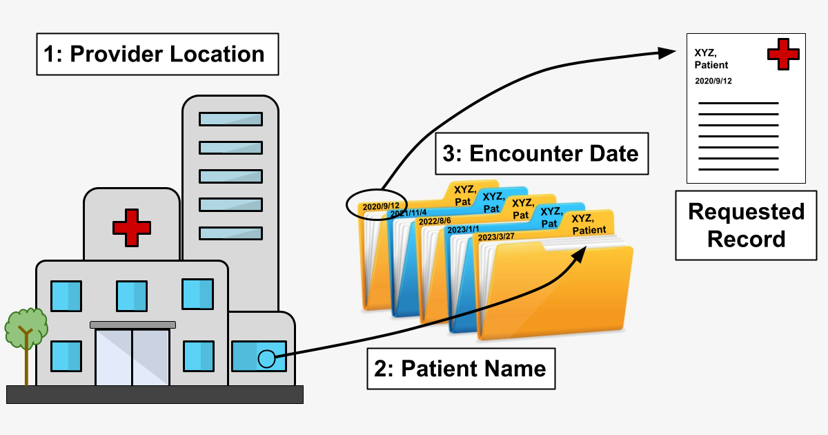
1. Provider information – We have information sufficient to know where to look for a record (Dr.’s office / hospital / clinic etc.), and we can either:
a.) retrieve the record manually (via fax, by sending a person to a physical location, etc.) or,
b.) retrieve the record digitally (via API call, through a 3rd-party EMR vendor, etc.).
2. Patient information – We know whose record we’re looking for.
3. Encounter date – Among the various records for a given patient at a given provider, we identify the correct record via the date the service was provided (an “Encounter”).
In a world of paper medical records, starting with the physical location of the provider and moving by steps toward the specific record would be the only way to proceed. (That is, you wouldn’t send somebody to Florida to find a record in Oregon.) Recreating a digital version of this path – “provider-based flow” – was a necessary first step in building a retrieval system at scale because even though provider “file cabinets” are increasingly digital, they are not necessarily connected in highly useful ways.
When there isn’t enough information
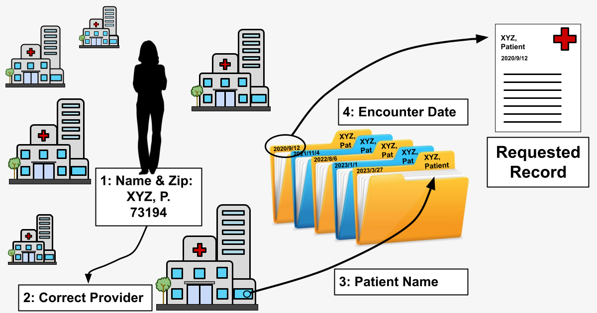
Datavant often receives requests, however, for which we don’t have information sufficient to carry out the provider-based flow route. If the record requester only gives us a patient name and an encounter date, we wouldn’t know where to start looking for the record. We’ve described this problem elsewhere as the “finding a needle in an invisible haystack” problem. In order to locate a record under these circumstances, Datavant has developed a route forperson-based flow.
Person-based flow is already in use in our Convenet product in England, something made possible because of England’s centralized health system and Convenet’s integration with the NHS-Spine. The problem in the US is much more challenging because of the extreme fragmentation and siloing of our healthcare landscape. To continue the above metaphor, there are many, many “invisible haystacks’’ across the American healthcare ecosystem where records could be stored.
Setting the parameters for person-based flow
Because requests may have varying levels of patient data included in them, the actual routing component of the service should be able to operate on a minimum amount of information, which we have determined to be the patient’s name and zip code as registered with their insurance company.
We can think of building person-based flow as creating a superset of provider-based flow:
Because we need to make API calls to several providers to locate a record, our routing mechanism must downselect from hundreds of connected clinics to only those most likely to contain the patient’s medical record. Obviously we can’t simply flood every provider in our network with all 50 million record requests, but more than that, we want to go as far as possible toward reducing our load on client API services. In fulfilling our mission to connect health data and improve patient outcomes, we want to keep our request loads on healthcare provider systems as light as possible.
Finding a haystack in a field of haystacks
For the rest of this article, we’ll use “clinic” to refer to any location where a patient may have received medical care and a medical record might be found.
Our person-based flow routing uses an approach that combines Thompson Sampling (TS) with k-nearest neighbors (KNN).
In our case, our “casino” is the size of the entire United States.
Thompson Sampling
Thompson Sampling is a Bayesian decision-making heuristic where actions are taken sequentially in a manner that must balance between exploiting what is known to maximize immediate performance and investing to accumulate new information that may improve future performance (balancing exploitation vs. exploration). This is also known as an algorithm for choosing the actions that address the exploration-exploitation dilemma in the multi-armed bandit problem.
Instead of deciding which arm to pull next on a group of slot machines, here we balance exploiting popular clinics that have a high probability of containing a patient’s medical record with exploring other clinics that have a yet to be determined or high variance probability of containing a patient’s medical record. And in our case, our “casino” is the size of the entire United States.
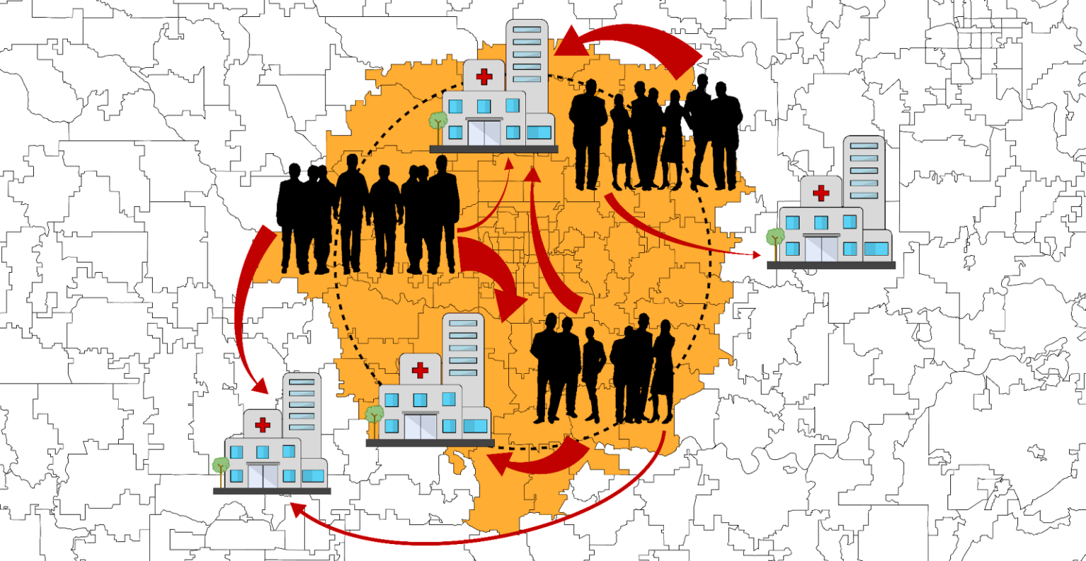
To our advantage, however, there is a geo-spatial relationship between our players (patients) and the expected reward of the slot machines (the likelihood of a clinic having a chart). We use KNN to exploit this fact and build priors intelligently (beginning distributions that model a clinic having a chart given a patient postal code).
K-nearest-neighbors
K-nearest neighbors is a supervised learning method to select a rank-ordered list based on a distance metric. In this case, our distance metric is the cartesian “as-the-crow-flies” distance between postal codes. This allows us to cast a wider net of historical information when profiling the care habits of patients living within a postal code. Put another way, KNN allows the algorithm to leverage nearby postal code information when current postal code information is scarce, and does so by assuming that patients living in adjacent or nearby postal codes will have similar care habits.
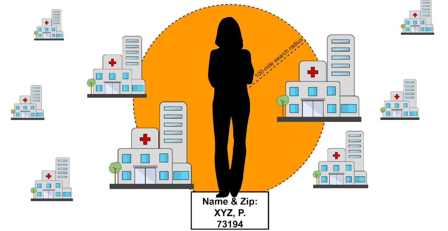
Benchmarking with DS algorithm
We tested the performance of two algorithms: modified-TS, described in detail below, and a simple Distance Heuristic (DS) to be used as a benchmark. The default setting for the DS algorithm was to return any clinic within 100 miles of the patient zip code:
Designing our modified-TS approach
Our “modified-TS” approach can be summarized in four steps.
After receiving the patient postal code as an input, we:
1. Create a bucket of 100 closest postal codes to the patient (KNN).
2. Model Probability Distribution Functions (PDFs*) for clinic-postal code pairs (TS).
3. Sample patient-clinic PDFs then weight average and rank order clinic scores (TS).
4. Send clinics above 3% probability to our Dispatcher tool (the routing service responsible for coordinating jobs).
*not to be confused with Portable Document Format
Let’s break that down.
Step 1: Create a bucket of 100 nearest postal codes to the patient
The first step of the modified-TS algorithm is to form a group of 100* nearest postal codes to the patient’s postal code, referred to as a “bucket.” The bucket leverages similarities in clinic visit behavior between patients who live near one another. It also allows the algorithm to model a probability for a patient living in a postal code for which there is little to no information. The bucket weights are uniform, meaning the historical data taken from every postal code in the bucket has equal voting rights.
*We tested variable distances for a hard mileage-based cutoff, as well as various numbers of k-nearest neighbors; K=100 was found to be optimal.
Step 2: Model Probability Distribution Functions (PDFs) for clinic-postal code pairs
The second step of the modified-TS algorithm is to model PDFs of each clinic-postal pair. The chosen PDF for this was the beta distribution, which models probability based on the success and failure of every chart request received by a clinic for a given patient postal code. Typically, historical information can be leveraged via simulation whereby distribution parameters are updated according to Bayes’ rule. This simulation however, is computationally expensive, as Datavant processes many years’ worth of record retrieval data (hundreds of millions of records).
Instead, the following analytical approach was employed to solve for the parameters of the respective beta distributions for every clinic-postal pair:
- Success (alpha) was taken as the count of total charts retrieved from the clinic from its paired postal code.
- Failure (beta) was taken as the total number of charts found for the paired postal code, minus alpha.
Step 3: Sample patient-clinic PDFs, then weight average and rank order clinic scores
The sampling of the PDFs is what allows for the exploration-exploitation tradeoff in the traditional TS approach. The rank order step ensures that priority is given to clinics with a high expected value, but that clinics with a lower expected value and high variance are occasionally selected as well. After sampling from the PDFs, an equally weighted (flat) average is taken for clinics represented by multiple postal codes.
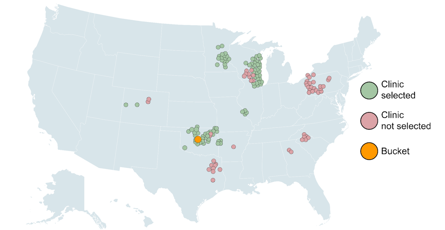
Step 4: Send clinics above 3% probability to Dispatcher
In the final step, the highest probability clinics (those above a 3% minimum cutoff) are sent to Dispatcher. Keep in mind that the algorithm is not limited to returning clinics within 100 miles of the patient: we can return clinics anywhere within the U.S. as long as there is historical data of patients traveling from the bucket to the respective clinic.
Fine tuning the model: adding hyperparameters
Four hyperparameters were selected for the modified-TS algorithm: K in KNN (the bucket size), starting_context_scale (the weight given to surrounding postal codes), max_returns (the hard number of top clinics to return), and prob_min (the minimum probability by which a clinic is selected).
We won’t go into all of the details of those here, but an extensive primary gridsearch was performed to give 54 unique combinations of hyperparameters. Upon selection of max_distance, starting_context_scale, and max_returns, a more selective, secondary gridsearch was performed to optimize prob_min. The results of the secondary gridsearch are shown below.
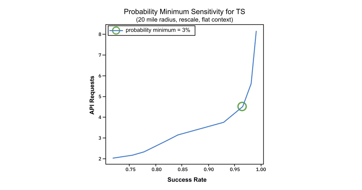
API Requests and Success Rate are plotted against one another. The “elbow” indicated by the green circle, indicates that at a prob_min setting of 3%, the relationship between success rate and API requests begins to degrade, requiring many more API calls to achieve a very modest increase in success.
The final selected values for the hyperparameters correspond to a 95% success rate and 7.2 average API calls on a 10K test dataset.
Avoiding bias: contextualizing bucket weights
When grouping patients into buckets, KNN by itself does not take into account transit obstructions like waterways and large highways, nor does it consider the availability of public transit, income demographics or other variables that might affect the likelihood of proximal patients having similar care habits. To circumvent this, we ran an additional experiment.
In simulations limited to individual cities in the database, the modified-TS algorithm was allowed to store and update the weights between postal codes stored in the bucket (see Step 1, above) in a gradient descent-like fashion. This demonstrated dramatic improvement over the standard Bayes’ rule approach:
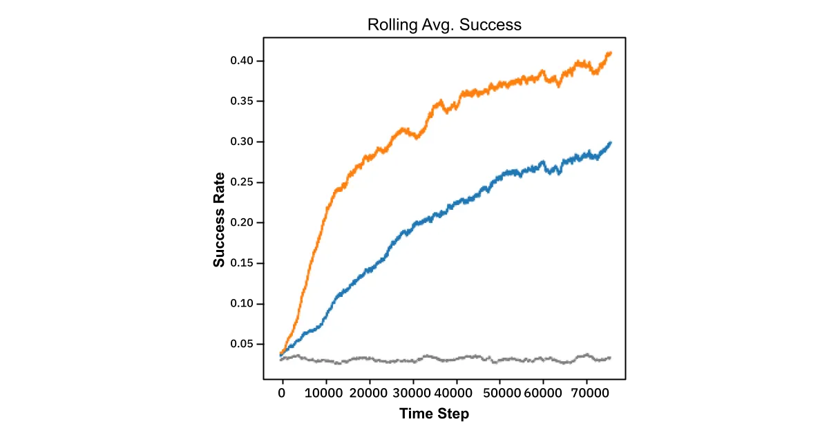
In other words, by pairing KNN with a learned weighting strategy the algorithm rewards nearby postals that return correct predictions and discounts those that don’t. So regardless of the underlying reason for different care habits, the model learns these effects at the granularity level of postal code. This experiment was performed for the cities of Saint Louis, Pittsburg, Milwaukee, NYC, Louisville, and Lexington, all with similar results. Mathematical details of this approach are available in the appendix.
Results
Results of our comparison test are shown below. The 10K test dataset was identical for both algorithms (none of which was used in training for the modified-TS algorithm). Success was determined as whether the actual clinic in the test dataset was returned in the clinic list produced by the algorithm.
- The success rate is the average of this binary output.
- The API calls is taken as the number of clinics produced in the clinic list by the algorithm – it is an indication of the downstream resources required to fulfill the request (lower is better).
- The performance is the computational time required for each algorithm to produce one clinic list for a patient postal code on an M1 laptop.
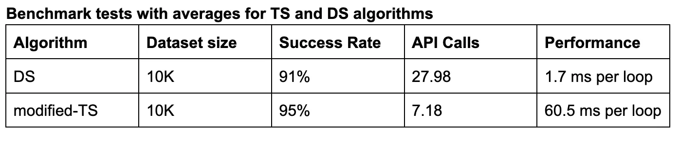
There was a decent lift in success rate, from 91% to 95%, and an enormous reduction in API calls, from 27.98 down to 7.18. Our modified-TS approach will likely lead to a slight increase in more patient charts retrieved but at a substantially lower resource cost.
Conclusion
Our expansion from provider-based flow to person-based flow allows us to find more medical records with less information. Combined with our recent API retrieval optimization, our combined-algorithm approach expedites record retrieval at scale, and allows us to do so in a way that minimizes the burden placed on the care providers receiving our requests. In the end, this allows us to improve patient outcomes directly for the patients trying to get their records in the course of care, and indirectly by allowing providers to allocate limited resources (computing power) where it is most needed, at the location of treatment.
Appendix
Mathematical Details
Glossary
ð‘‹ : the context coefficient matrix (referred to as a bucket in the main document)
𜃠: estimated success probabilities
ð‘¡ : current time step
ð‘ : available regions (postal codes)
𑘠: available targets/actions (facilities)
ð‘¥ð‘¡ : the target selected/action taken
ð‘¦ð‘¡ : the current region
ð‘Ÿð‘¡ : the reward of selected target (0 or 1)
𛼠: alpha parameter of the beta distribution
𛽠: beta parameter of the beta distribution
𜂠: context learning rate
Theta, the PDFs
The update criteria for ðœƒ, the object that stores the weights of the beta distributions:

X, the postal-postal buckets
The update criteria for X, the object that stores the postal postal buckets:

About the Authors
Authored by Wesley Beckner and Nicholas DeMaison, with input from Ryan Ma, Jonah Leshin, Arjun Sanghvi, Aneesh Kulkarni, and Shannon West.
Wesley Beckner holds a PhD in Chemical Engineering Data Science from the University of Washington College of Engineering and is a Data Scientist for Datavant. Connect with Wesley on LinkedIn.
Ryan Ma has a background in Computer Science and Molecular and Cell Biology. He is a Software Engineer for Datavant. Connect with Ryan on LinkedIn.
Nicholas DeMaison writes for Datavant where he leads talent branding initiatives. Connect with Nick on LinkedIn.
We’re hiring remotely across teams. Check out our open positions.

